DCGAN

The fully connected GAN that we implemented in the last section generated MNIST images of subpar quality. This is to be expected, because plain vanilla fully connected neural networks are not well suited for images. Instead we usually utilize convolutional neural networks, if we want to achieve good performance in the area of computer vision. DCGANs[1] (deep convolutional generative adversarial networks) do just that by using CNNs for the generator and discriminator.

The generator takes a latent vector as input. We follow the original implementation and use a noise of size 100. This noise is interpreted as 100 feature maps of size 1x1, so each input is of size 100x1x1. The noise is processed by layers of transposed convolutions, batch norm and rectified linear units. Transposed convolutions upscale the images and reduce the number of channels, until we end up with images of size 1x64x64. The dimensionality of 64 was picked for convenience in order to follow the original parameters from the paper. We will once again work with MNIST, but we upscale the images to 64x64.

class Generator(nn.Module):
    def __init__(self):
        super().__init__()
        self.generator = nn.Sequential(
            nn.ConvTranspose2d(
                in_channels=LATENT_SIZE, out_channels=1024, kernel_size=4, bias=False
            ),
            nn.BatchNorm2d(1024),
            nn.ReLU(),
            nn.ConvTranspose2d(
                in_channels=1024,
                out_channels=512,
                kernel_size=4,
                padding=1,
                stride=2,
                bias=False,
            ),
            nn.BatchNorm2d(512),
            nn.ReLU(),
            nn.ConvTranspose2d(
                in_channels=512,
                out_channels=256,
                kernel_size=4,
                padding=1,
                stride=2,
                bias=False,
            ),
            nn.BatchNorm2d(256),
            nn.ReLU(),
            nn.ConvTranspose2d(
                in_channels=256,
                out_channels=128,
                kernel_size=4,
                padding=1,
                stride=2,
                bias=False,
            ),
            nn.BatchNorm2d(128),
            nn.ReLU(),
            nn.ConvTranspose2d(
                in_channels=128,
                out_channels=1,
                kernel_size=4,
                padding=1,
                stride=2,
                bias=True,
            ),
            nn.Tanh(),
        )

    def forward(self, x):
        return self.generator(x)

The discriminator on the other hand takes images as input and applies layers of convolutions. This procedure increases the number of channels and downscales the images. The last layer reduces the number of channels to 1 and ends up with images of size 1x1x1. This value is flattened and is used as input for sigmoid in order to be interpreted as probability of being a real image.

class Discriminator(nn.Module):
    def __init__(self):
        super().__init__()
        self.discriminator = nn.Sequential(
            nn.Conv2d(
                in_channels=1,
                out_channels=128,
                kernel_size=4,
                padding=1,
                stride=2,
                bias=True,
            ),
            nn.LeakyReLU(0.2),
            nn.Conv2d(
                in_channels=128,
                out_channels=256,
                kernel_size=4,
                padding=1,
                stride=2,
                bias=False,
            ),
            nn.BatchNorm2d(256),
            nn.LeakyReLU(0.2),
            nn.Conv2d(
                in_channels=256,
                out_channels=512,
                kernel_size=4,
                padding=1,
                stride=2,
                bias=False,
            ),
            nn.BatchNorm2d(512),
            nn.LeakyReLU(0.2),
            nn.Conv2d(
                in_channels=512,
                out_channels=1024,
                kernel_size=4,
                padding=1,
                stride=2,
                bias=False,
            ),
            nn.BatchNorm2d(1024),
            nn.LeakyReLU(0.2),
            nn.Conv2d(
                in_channels=1024,
                out_channels=1,
                kernel_size=4,
                padding=0,
                stride=1,
                bias=True,
            ),
            nn.Flatten(),
        )

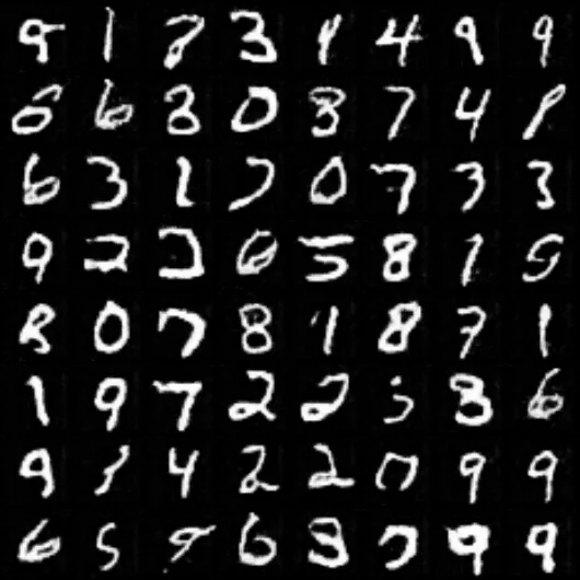
When we train a DCGAN for 20 epochs we end with the following results. The images are more realistic and there are fewer artifacts compared to those from the last section.