Dropout

Dropout is a regularization technique, that was developed by Geoffrey Hinton and his colleagues at the university of Toronto [1] [2] .

You can use the interactive example below. We use a relatively small neural network below and apply dropout with a p undefined value of 0.2 to the two hidden layer.

Theoretically you can apply dropout to any layer you desire, but most likely you will not want to deactivate the input and the output layers.

When we use our model for inference, we do not remove any of the nodes randomly. If we did that, we would get different results each time we run a model. By not deactivating any nodes we introduce a problem though. More neurons are active during inference, therefore each layer has to deal with an input that is on a different scale, than the one the neural network has seen during training. Different conditions during training and inference will prevent the neural network from generating good predictions. To prevent that from happening the active nodes are scaled by \dfrac{1}{1-p} undefined during training, which increases the magnitude of the input signal. We skip that scaling during inference, but the average signal strength remains fairly similar, as the network now has more neurons as inputs.

Let us assume for example that a layer of neurons contains only 1's and p undefined is 0.5.

The dropout layer will zero out roughly half of the activations and multiply the rest by \dfrac{1}{1-0.5} = 2 undefined .

But why is the dropout procedure helpful in avoiding overfitting? Each time we remove a set of neurons from training, we essentially create a different, simplified model. This simplified model has to learn to deal with the task at hand without overrelying on any of the neurons from the previous layer, because any of those might get deactivated at any time. The final model can be seen as an ensemble of an immensely huge collection of simplified models. Ensembles tend to produce better results and reduce overfitting. You will notice that in practice dropout works extremely well.

As expected PyTorch provides built-in nn.Dropout() modules with a probability parameter p. We add those after each of the hidden layers and we are good to go.

class Model(nn.Module):
    def __init__(self):
        super().__init__()
        self.layers = nn.Sequential(
                nn.Flatten(),
                nn.Linear(NUM_FEATURES, HIDDEN_SIZE_1),
                nn.Sigmoid(),
                nn.Dropout(p=0.6),
                nn.Linear(HIDDEN_SIZE_1, HIDDEN_SIZE_2),
                nn.Sigmoid(),
                nn.Dropout(p=0.6),
                nn.Linear(HIDDEN_SIZE_2, NUM_LABELS),
            )
    
    def forward(self, features):
        return self.layers(features)

There are a couple more adjustments we need to make, to actually make our code behave the way we desire. We can set modules in training and evaluation modes. Modules might behave differently, depending on the mode they are in. As mentioned before dropout needs to behave differently depending on whether we are training or evaluating, but there are more layers in PyTorch, that require that distinction.

To actually set the modules in different modes is actually qute easy. Below we use model.eval() to start evaluation mode at the start of the function.

def track_performance(dataloader, model, criterion):
    # switch to evaluation mode
    model.eval()

    num_samples = 0
    num_correct = 0
    loss_sum = 0
    
    # no need to calculate gradients
    with torch.inference_mode():
        for batch_idx, (features, labels) in enumerate(dataloader):
            features = features.view(-1, NUM_FEATURES).to(DEVICE)
            labels = labels.to(DEVICE)
            logits = model(features)
            
            predictions = logits.max(dim=1)[1]
            num_correct += (predictions == labels).sum().item()
            
            loss = criterion(logits, labels)
            loss_sum += loss.cpu().item()
            num_samples += len(features)
    
    # we return the average loss and the accuracy
    return loss_sum/num_samples, num_correct/num_samples

The method model.train() on the other hand puts all the modules in training mode.

def train_epoch(dataloader, model, criterion, optimizer):
    # switch to training mode
    model.train()
    for batch_idx, (features, labels) in enumerate(train_dataloader):
        # move features and labels to GPU
        features = features.to(DEVICE)
        labels = labels.to(DEVICE)

        # ------ FORWARD PASS --------
        output = model(features)

        # ------CALCULATE LOSS --------
        loss = criterion(output, labels)

        # ------BACKPROPAGATION --------
        loss.backward()

        # ------GRADIENT DESCENT --------
        optimizer.step()

        # ------CLEAR GRADIENTS --------
        optimizer.zero_grad()

model = Model().to(DEVICE)
criterion = nn.CrossEntropyLoss(reduction="sum")
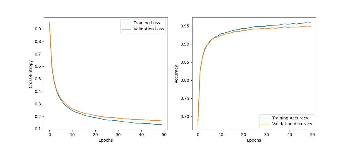
optimizer = optim.SGD(model.parameters(), lr=0.005)

There is still some distance between the performance of the training and the validation datasets, but we are manage to reduce overfitting by using dropout.

history = train(NUM_EPOCHS, train_dataloader, val_dataloader, model, criterion, optimizer)

Epoch: 1/50|Train Loss: 0.9384 |Val Loss: 0.9489 |Train Acc: 0.6870 |Val Acc: 0.6770
Epoch: 10/50|Train Loss: 0.2586 |Val Loss: 0.2698 |Train Acc: 0.9232 |Val Acc: 0.9202
Epoch: 20/50|Train Loss: 0.1905 |Val Loss: 0.2089 |Train Acc: 0.9427 |Val Acc: 0.9363
Epoch: 30/50|Train Loss: 0.1658 |Val Loss: 0.1869 |Train Acc: 0.9479 |Val Acc: 0.9417
Epoch: 40/50|Train Loss: 0.1450 |Val Loss: 0.1732 |Train Acc: 0.9547 |Val Acc: 0.9458
Epoch: 50/50|Train Loss: 0.1313 |Val Loss: 0.1624 |Train Acc: 0.9590 |Val Acc: 0.9483

plot_history(history, 'dropout_overfitting')