Activation Functions

The sigmoid activation function is one of the main causes of the vanishing gradients problem. Because of that researchers have tried to come up with activation functions with better properties. In this section we are going to compare and contrast some of the most popular activation functions, while emphasizing when each of the activations should be used.

Sigmoid and Softmax

From our previous discussion it might have seemed, that the sigmoid activation function (and by extension softmax) is the root cause of the vanishing gradient problem and should be avoided at all cost.

While this is somewhat true, the original argumentation that we used when we implemented logistic regression still applies. We can use the sigmoid and the softmax to turn logits into probabilities. Nowadays we primarily use the sigmoid \dfrac{1}{1+e^{-z}} undefined and the softmax \dfrac{e^{z}}{\sum e^{z}} undefined in the last layer of the neural network, to determine the probability to belong to a particular class.

There are generally two ways to implement activation functions. We can use PyTorch in a functional way and apply torch.sigmoid(X) in the forward() function of the model or as we have done so far, we can use the object-oriented way and use the torch.nn.Sigmoid() as part of nn.Sequential().

# functional way
sigmoid_output = torch.sigmoid(X)
# object-oriented way
sigmoid_layer = torch.nn.Sigmoid()

If we can fit the whole logic of the model into nn.Sequential, we will generally do that and use the object-oriented way. Sometimes, when the code gets more complicated, this will not possible and we will resort to the functional approach. The choice is generally yours.

Hyperbolic Tangent

The tanh activation function \dfrac{e^{z} - e^{-z}}{e^{z} + e^{-z}} undefined (also called hypterbolic tangent) is similar in spirit to the sigmoid activation function. Looking from a distance you might confuse the two, but there are some subtle differences.

While both functions saturate when we use very low and very high inputs, the sigmoid squishes values between 0 and 1, while the tanh squishes values between -1 and 1.

For a long time researchers used the tanh activation function instead of the sigmoid, because it worked better in practice. Generally tanh exhibits a more favourable derivative function. While the sigmoid can only have very low derivatives of up to 0.25, the tanh can exhibit a derivative of up to 1, thereby reducing the risk of vanishing gradients.

Over time researchers found better activations functoions that they prefer over tanh, but in case you actually desire outputs between -1 and 1, you should use the tanh.

Once again there are two broad approaches to activation functions: the functional and the object-oriented one.

tanh_output = torch.tanh(X)
tanh_layer = torch.nn.Tanh()

ReLU

The ReLU (rectified linear unit) is at the same time extremely simple and extremely powerful. The function returns the unchanged input z undefined as its output when the input value is positive and 0 otherwise [1] .

The calculation of the derivative is also extremely straightforward. It is exactly 1 when the net input z undefined is above 1 and 0 otherwise. While technically we can not differentiate the function at the knick, in practice this works very well.

Hopefully you will interject at this point and point out, that while the derivative of exactly 1 will help to fight the problem of vanishing gradients, a derivative of 0 will push the product in the chain rule to exactly 0. This is true and is known as the dying relu problem, but in practice you will not encounter the problem too often. Given that you have a large amount of neurons in each layer, there should be enough paths to propagate the signal.

PyTorch offers the two approaches for ReLU as well.

relu_output = torch.relu(X)
relu_layer = torch.nn.ReLU()

Over time researchers tried to come up with improvements for the ReLU activation. The leaky ReLU for example does not completely kill off the signal, but provides a small slope when the net input is negative.

In the example below alpha corresponds to 0.1.

When activation functions start to get slighly more exotic, you will often not find the in the torch namespace directly, but in the torch.nn.functional namespace.

lrelu_output = torch.nn.functional.leaky_relu(X, negative_slope=0.01)
lrelu_layer = torch.nn.LeakyReLU(negative_slope=0.01)

There are many more activation functions out there, expecially those that try to improve the original ReLU. For the most part we will use the plain vanilla ReLU, because the mentioned improvements generally do not provide significant advantages.

Now let's have a peak at the difference in the performance between the sigmoid and the ReLU activation functions. Once again we are dealing with the MNIST dataset, but this time around we create two models, each with a different set of activation functions. Both models are larger, than they need to be, in order to demonstrate the vanishing gradient problem.

class SigmoidModel(nn.Module):
    def __init__(self):
        super().__init__()
        self.layers = nn.Sequential(
            nn.Flatten(),
            nn.Linear(NUM_FEATURES, HIDDEN),
            nn.Sigmoid(),
            nn.Linear(HIDDEN, HIDDEN),
            nn.Sigmoid(),
            nn.Linear(HIDDEN, HIDDEN),
            nn.Sigmoid(),
            nn.Linear(HIDDEN, HIDDEN),
            nn.Sigmoid(),
            nn.Linear(HIDDEN, HIDDEN),
            nn.Sigmoid(),
            nn.Linear(HIDDEN, NUM_LABELS)
        )
        
    def forward(self, features):
        return self.layers(features)
    
class ReluModel(nn.Module):
    def __init__(self):
        super().__init__()
        self.layers = nn.Sequential(
            nn.Flatten(),
            nn.Linear(NUM_FEATURES, HIDDEN),
            nn.ReLU(),
            nn.Linear(HIDDEN, HIDDEN),
            nn.ReLU(),
            nn.Linear(HIDDEN, HIDDEN),
            nn.ReLU(),
            nn.Linear(HIDDEN, HIDDEN),
            nn.ReLU(),
            nn.Linear(HIDDEN, HIDDEN),
            nn.ReLU(),
            nn.Linear(HIDDEN, NUM_LABELS)
        )
        
    def forward(self, features):
        return self.layers(features)

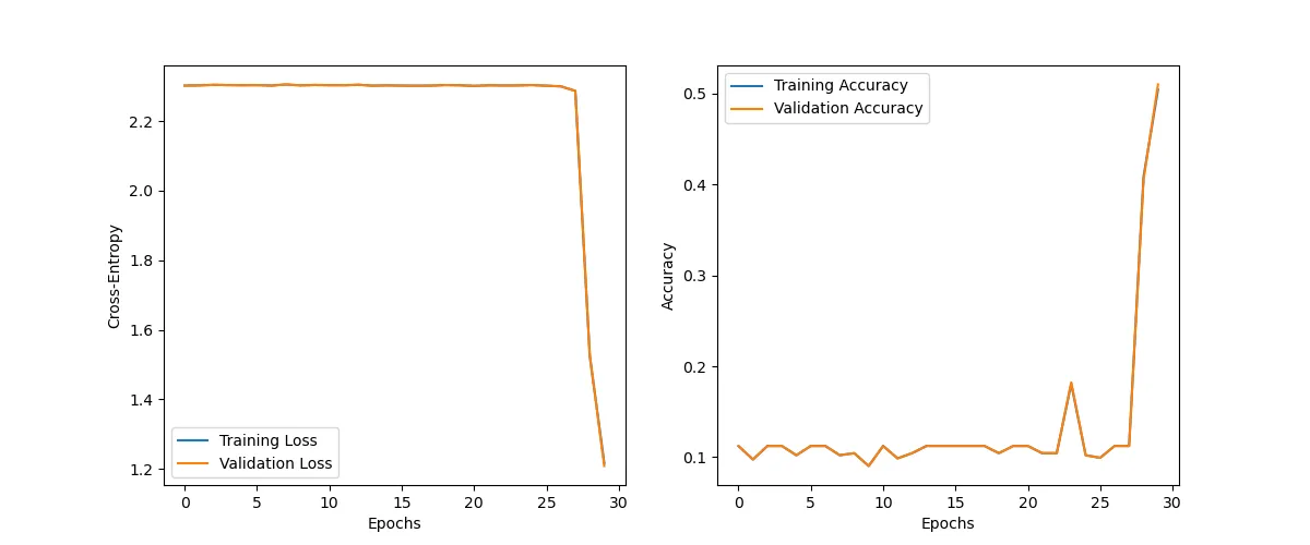
The sigmoid model starts out very slowly and even after 30 iterations has not managed to decrease the training loss significantly. If you train the same sigmoid model several times, you will notice, that sometimes the loss does not decrease at all. It all depends on the starting weights.

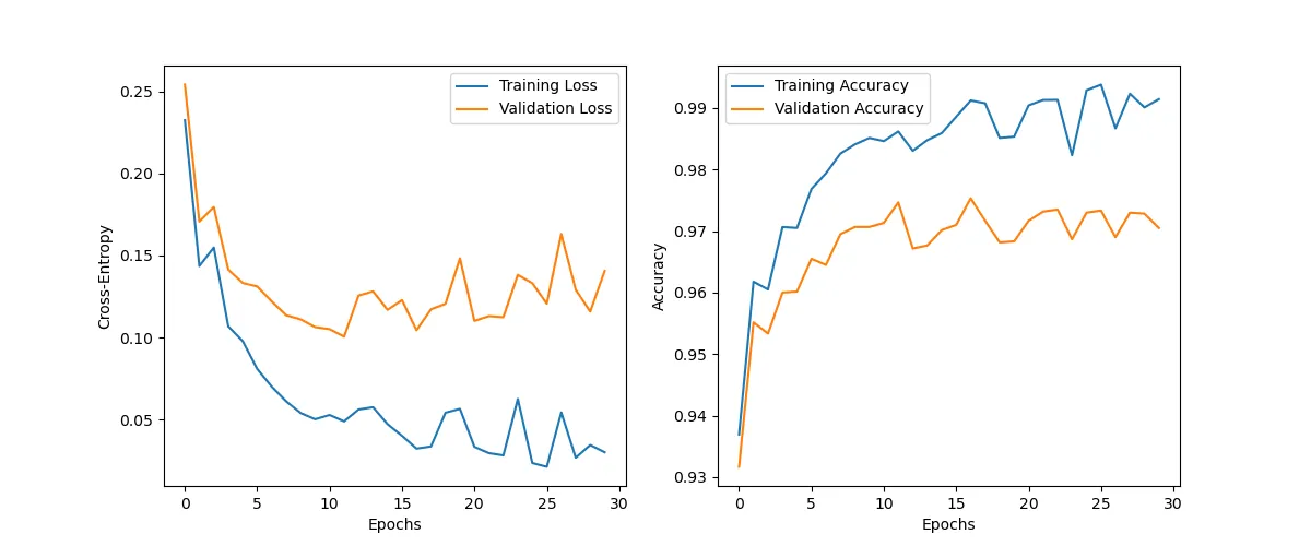
The loss of the ReLU model on the other hand decreases significantly, thus indicating that the gradients propagate much better with this type of activation function.