Regularization
The goal of regularization is to encourage simpler models. Simpler models can not fit the data exactly and are therefore less prone to overfitting. While there are several techniques to achieve that goal, in this section we focus on techniques that modify the loss function.
We will start this section by reminding ourselves of a term usually learned in an introductory linear algebra course, the norm. The norm measures the distance of a vector \mathbf{v} undefined from the origin. The p-norm (written L_p undefined ) for the vector \mathbf{v} undefined is defined as ||\mathbf{v}||_p = \large\sqrt{\sum_{i=1}^n |v_i|^p} undefined . By changing the parameter p undefined from 1 to infinity we get different types of norms. In machine learning and deep learning we are especially interested in the L_1 undefined and theL_2 undefined norm.
L2 Norm
The L_2 undefined norm also called Euclidean norm is the distance measure we are most familiar with. When we are given the vector \begin{bmatrix} 5 \\ 4 \end{bmatrix} undefined for example we can regard the number 5 as the x coordinate and the numver 4 as the y coordinate. As shown in the graph below this vector is essentially a hypotenuse of a right triangle, therefore we need to apply the Pythagorean theorem to calculate the length of the vector, c^2 = \displaystyle\sqrt{a^2 + b^2} undefined .
While the the Pythagorean theorem is used to calculate the length of a vector on a 2 dimensional plane, the L_2 undefined norm generalizes the idea of length to n undefined dimensions, ||\mathbf{v}||_2 =\displaystyle \sqrt{\sum_{i=1}^n v_i^2} undefined .
Now let's assume we want to find all vectors on a two dimensional plane that have a specific L_2 undefined norm of size l undefined . When we are given a specific vector length l undefined such that \displaystyle \sqrt{x_1^2 + x_2^2} = l undefined , we will find that there is whole set of vectors that satisfy that condition and that this set has a circular shape. In the interactive example below we assume that the norm is 1, \displaystyle \sqrt{x_1^2 + x_2^2} = 1 undefined . If we draw all the vectors with the norm of 1 we get a unit circle.
There is an infinite number of such circles, each corresponding to a different set of vectors with a particular L_2 undefined norm. The larger the radius, the larger the norm. Below we draw the circles that correspond to the L_2 undefined norm of 1, 2 and 3 respectively.
Now let's try and anderstand how this visualization of a norm can be useful. Imagine we are given a single equation x_1 + x_2 = 3 undefined . This is an underdetermined system of equations, because we have just 1 equation and 2 unknowns. That means that there is literally an infinite number of possible solutions. We can depict the whole set of solutions as a single line. Points on that line show combinations of x_1 undefined and x_2 undefined that sum up to 3.
Below we add the norm for the x_1 undefined , x_2 undefined vector. The slider controls the size of the L_2 undefined norm. When you keep increasing the norm you will realize that at the red point the circle is going to just barely touch the line. At this point we see the solution for x_1 + x_2 = 3 undefined that has the smallest L2 undefined norm out of all possible solutions.
If we are able to find solutions that have a comparatively low L_2 undefined how does this apply to machine learning and why is this useful to avoid overfitting? We can add the squared L_2 undefined norm to the loss function as a regularizer. We do not use the ||L||_2 undefined norm directly, but calculate the square of the norm, ||L||_2^2 undefined , because the root makes the calculation of the derivative more complicarted than it needs to be.
If we are dealing with the mean squared error for example, our new loss function looks as below.
L=\dfrac{1}{n}\sum_i^n (y^{(i)} - \hat{y}^{(i)} )^2 + \lambda \sum_j^m w_j^2 undefinedThe overall intention is to find the solution that reduces the mean squared error without creating large weights. When the size of one of the weights increses disproportionatly, the regularization term will increase and the loss function will rise sharply. In order to avoid a large loss, gradient descent will push the weights closer to 0. Therefore by using the regularization term we reduce the size of the weights and the overemphasis on any particular feature, thereby reducing the complexity of the model. The \lambda undefined (lambda) is the hyperparameter that we can tune to determine how much emphasis we would like to put on the L_2 undefined norm. It is the lever that lets you control the size of the weights.
Below we have the same model trained with and without the L_2 undefined regurlarization. You can move the slider to adjust the lambda. The higher the lambda, the simpler the model becomes and the more the curve looks like a straight line.
We can implement L_2 undefined regularization in PyTorch, by adding a couple more lines to our calculation of the loss function. Esentially we loop over all weights and biases, square those and calculate a sum. Autograd does the rest.
LAMBDA = 0.01
def train_epoch(dataloader, model, criterion, optimizer):
    for batch_idx, (features, labels) in enumerate(train_dataloader):
        # move features and labels to GPU
        features = features.to(DEVICE)
        labels = labels.to(DEVICE)

        # ------ FORWARD PASS --------
        output = model(features)

        # ------CALCULATE LOSS --------
        loss = criterion(output, labels)
        l2 = None
        for param in model.parameters():
            if l2 is None:
                l2 = param.pow(2).sum()
            else:
                l2 += param.pow(2).sum()

        loss += LAMBDA * l2

        # ------BACKPROPAGATION --------
        loss.backward()

        # ------GRADIENT DESCENT --------
        optimizer.step()

        # ------CLEAR GRADIENTS --------
        optimizer.zero_grad()
model = Model().to(DEVICE)
criterion = nn.CrossEntropyLoss(reduction="sum")
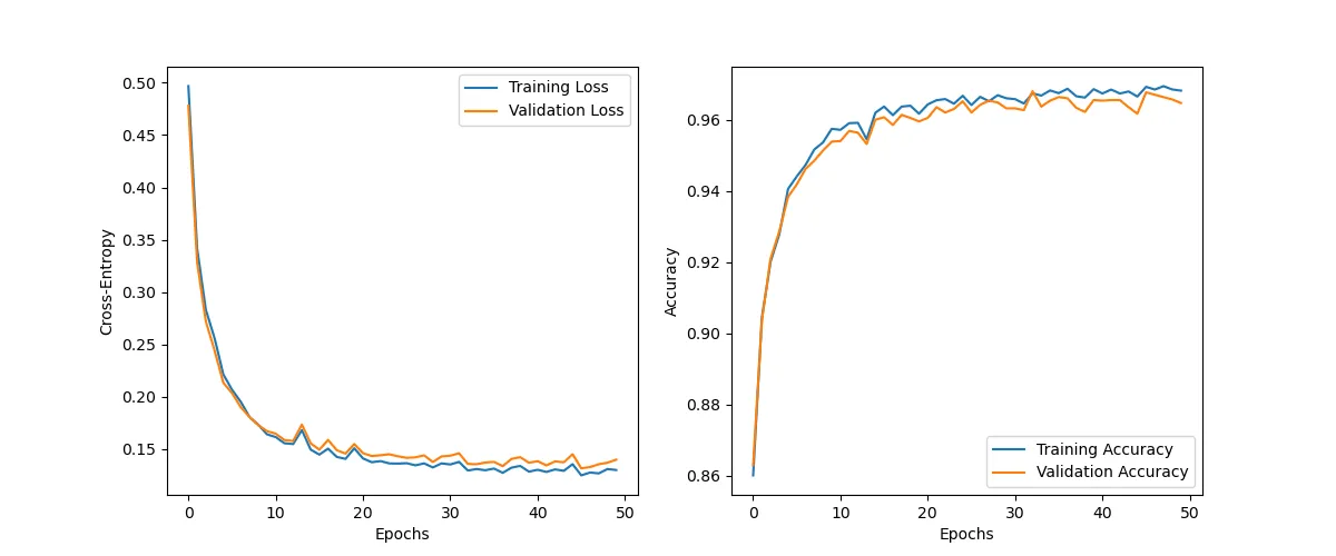
optimizer = optim.SGD(model.parameters(), lr=0.005)Our regularization procedure does a fine job reducing overfitting.
history = train(NUM_EPOCHS, train_dataloader, val_dataloader, model, criterion, optimizer)Epoch: 1/50|Train Loss: 0.4967 |Val Loss: 0.4781 |Train Acc: 0.8601 |Val Acc: 0.8630
Epoch: 10/50|Train Loss: 0.1641 |Val Loss: 0.1671 |Train Acc: 0.9574 |Val Acc: 0.9538
Epoch: 20/50|Train Loss: 0.1508 |Val Loss: 0.1548 |Train Acc: 0.9617 |Val Acc: 0.9595
Epoch: 30/50|Train Loss: 0.1363 |Val Loss: 0.1430 |Train Acc: 0.9660 |Val Acc: 0.9632
Epoch: 40/50|Train Loss: 0.1284 |Val Loss: 0.1369 |Train Acc: 0.9686 |Val Acc: 0.9655
Epoch: 50/50|Train Loss: 0.1300 |Val Loss: 0.1399 |Train Acc: 0.9681 |Val Acc: 0.9647

PyTorch actually provides a much easier way to implement L_2
undefined
regularization.
When you define your optimizer, you can pass the weight_decay
parameter. This is essentially the \lambda
undefined
from our equation above.
optimizer = optim.SGD(model.parameters(), lr=0.005, weight_decay=0.001)L1 Norm
The L_1 undefined norm, also called the Manhattan distance, simply adds absolute values of each element of the vector, ||\mathbf{v}||_1 = \sum_{i=1}^n |v_i| undefined .
This definition means essentially that when you want to move from the blue point to the red point, you do not take the direct route, but move along the axes.
We can make the same exercise we did with the L_2 undefined norm and imagine how the set of vectors looks like if we restrict the L_1 undefined norm to length 1 undefined : |x_1| + |x_2| = 1 undefined . The result is a diamond shaped figure. All vectors on the ridge of the diamond have a L_1 undefined norm of exactly 1.
Different L_1 undefined norms in 2D produce diamonds of different sizes.
Below we are given an underdetermined system of equations 2x_1 + x_2 = 3 undefined and we want to find a solution with the smallest L_1 undefined norm.
When you move the slider you will find the solution, where the diamond touches the line. This solution produces the vector with the lowest L_1 undefined norm. An important characteristic of the L_1 undefined norm is the so called sparse solution. The diamond has four sharp points. Each of those points corresponds to a vector where only one of the vector elements is not zero (this is also valid for more than two dimensions). That means that when the diomond touches the function, we are faced with a solution where the vector is mostly zero, a sparse vector.
When we add the L_1 undefined regularization to the mean squared error, we are simultaneously reducing the mean squared error and reduce the L_1 undefined norm. Similar to L_2 undefined , the L_1 undefined regularization reduces overfitting by not letting the weights grow disproportionatly. Additionally the L_1 undefined norm tends to generate sparse weights. Most of the weights will correspond to 0.
L=\frac{1}{n}\sum_i^n (y^{(i)} - \hat{y}^{(i)} )^2 + \lambda \sum_j^m |w_j| undefinedWe can implement L_1 undefined regularization, but adjusting our loss function slightly. The rest of the implementation is the same.
LAMBDA = 0.01
def train_epoch(dataloader, model, criterion, optimizer):
    for batch_idx, (features, labels) in enumerate(train_dataloader):
        # move features and labels to GPU
        features = features.to(DEVICE)
        labels = labels.to(DEVICE)

        # ------ FORWARD PASS --------
        output = model(features)

        # ------CALCULATE LOSS --------
        loss = criterion(output, labels)
        l1 = None
        for param in model.parameters():
            if l1 is None:
                l1 = param.abs().sum()
            else:
                l1 += param.abs().sum()

        loss += LAMBDA * l1

        # ------BACKPROPAGATION --------
        loss.backward()

        # ------GRADIENT DESCENT --------
        optimizer.step()

        # ------CLEAR GRADIENTS --------
        optimizer.zero_grad()
model = Model().to(DEVICE)
criterion = nn.CrossEntropyLoss(reduction="sum")
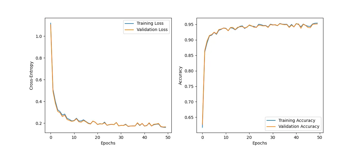
optimizer = optim.SGD(model.parameters(), lr=0.005)history = train(NUM_EPOCHS, train_dataloader, val_dataloader, model, criterion, optimizer)Epoch: 1/50|Train Loss: 1.1206 |Val Loss: 1.1060 |Train Acc: 0.6172 |Val Acc: 0.6270
Epoch: 10/50|Train Loss: 0.2200 |Val Loss: 0.2162 |Train Acc: 0.9383 |Val Acc: 0.9377
Epoch: 20/50|Train Loss: 0.2077 |Val Loss: 0.2087 |Train Acc: 0.9416 |Val Acc: 0.9405
Epoch: 30/50|Train Loss: 0.1744 |Val Loss: 0.1745 |Train Acc: 0.9507 |Val Acc: 0.9495
Epoch: 40/50|Train Loss: 0.1966 |Val Loss: 0.1966 |Train Acc: 0.9416 |Val Acc: 0.9417
Epoch: 50/50|Train Loss: 0.1604 |Val Loss: 0.1656 |Train Acc: 0.9541 |Val Acc: 0.9513
plot_history(history, 'l1_overfitting')