Data Augmentation

One of the best ways to reduce the chances of overfitting is to gather more data. Let's assume that we are dealing with MNIST and want to teach a neural net to recognize handwritten digits. If we provide the neural network with just ten images for training, one for each category, there is a very little chance, that the network will generalize and actually learn to recognize the digits. Instead it will memorize the specific samples. If we provide the network with millions of images on the other hand, the network has a smaller chance to memorize all those images.

MNIST provides 60,000 training images and 10,000 test images. This data is sufficient to train a good performing neral network, because the task is comparatively easy. In modern day deep learning this amount of data would be insufficient and we would be required to collect more data. Oftentimes collection of additional samples is not feasable and we will resort to data augmentation.

We can for example rotate, blur or flip the images, but there are many more options available. You can have a look at the PyTorch documentation to study the available options.

It is not always the case that we would take the 60,000 MNIST training samples, apply let's say 140,000 transformations and end up with 200,000 images for training. Often we apply random transformations to each batch of traning that we encounter. For example we could slightly rotate and blur each of the 32 images in our batch using some random parameters. That way our neural network never encounters the exact same image twice and has to learn to generalize. This the approach we are going to take with PyTorch.

We are going to use the exact same model and training loop, that we used in the previous section, so let us focus on the parts that acutally change.

We create a simple function, that saves and displays MNIST images.

# function to loop over a list of images and to draw them using matplotlib
def draw_images(images, name):
    fig = plt.figure(figsize=(10, 10))
    for i, img in enumerate(images):
        fig.add_subplot(1, len(images), i+1)
        img = img.squeeze()
        plt.imshow(img, cmap="gray")
        plt.axis('off')
    plt.savefig(f'{name}.png', bbox_inches='tight')
    plt.show()

First we generate 6 non-augmented images from the training dataset.

# original images
images = [train_validation_dataset[i][0] for i in range(6)]
draw_images(images, 'minst_orig')

We can rotate the images by using T.RandomRotation. We use an angle between -30 and 30 degrees to get the following results.

# rotate
transform = T.RandomRotation(degrees=(-30, 30))
transformed_images = [transform(img) for img in images]
draw_images(transformed_images, 'mnist_rotated')

We can blur the images by using T.GaussianBlur.

# gaussian blur
transform = T.GaussianBlur(kernel_size=(5,5))
transformed_images = [transform(img) for img in images]
draw_images(transformed_images, 'mnist_blur')

Or we can randomly flip the images by using T.RandomHorizontalFlip.

# flip
transform = T.RandomHorizontalFlip(p=1)
transformed_images = [transform(img) for img in images]
draw_images(transformed_images, 'mnist_flipped')

There are many more different augmentation transforms available, but in this example we will only apply one. First apply gaussian blur to the PIL image and then we transform the result into a PyTorch tensor.

transform = T.Compose([
    T.GaussianBlur(kernel_size=(5,5)),
    T.ToTensor(),
])

As we have created new transforms, we have to to create a new training dataset and dataloader.

train_validation_dataset_aug = MNIST(root="../datasets/", train=True, download=True, transform=transform)
train_dataset_aug = Subset(train_validation_dataset_aug, train_idxs)
val_dataset_aug = Subset(train_validation_dataset_aug, val_idxs)


train_dataloader_aug = DataLoader(dataset=train_dataset_aug, 
                              batch_size=BATCH_SIZE,
                              shuffle=True,
                              drop_last=True,
                              num_workers=4)
train_dataloader_aug = DataLoader(dataset=val_dataset_aug, 
                              batch_size=BATCH_SIZE,
                              shuffle=False,
                              drop_last=False,
                              num_workers=4)

It turns out that the learning rate that we used before is too large if we apply augmentations, so we use a reduced learning rate.

model = Model().to(DEVICE)
criterion = nn.CrossEntropyLoss(reduction="sum")
optimizer = optim.SGD(model.parameters(), lr=0.005)

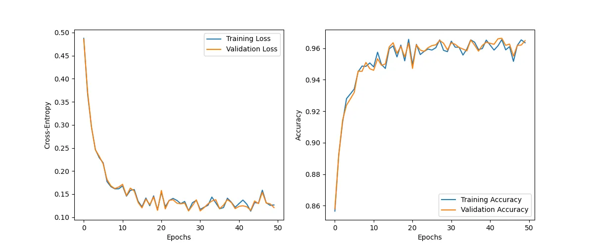
By using augmentation we reduce overfitting significantly.

history = train(NUM_EPOCHS, train_dataloader_aug, train_dataloader_aug, model, criterion, optimizer)

Epoch: 1/50|Train Loss: 0.4877 |Val Loss: 0.4859 |Train Acc: 0.8565 |Val Acc: 0.8580
Epoch: 10/50|Train Loss: 0.1616 |Val Loss: 0.1652 |Train Acc: 0.9507 |Val Acc: 0.9470
Epoch: 20/50|Train Loss: 0.1158 |Val Loss: 0.1149 |Train Acc: 0.9657 |Val Acc: 0.9633
Epoch: 30/50|Train Loss: 0.1366 |Val Loss: 0.1377 |Train Acc: 0.9578 |Val Acc: 0.9590
Epoch: 40/50|Train Loss: 0.1215 |Val Loss: 0.1187 |Train Acc: 0.9652 |Val Acc: 0.9638
Epoch: 50/50|Train Loss: 0.1265 |Val Loss: 0.1209 |Train Acc: 0.9635 |Val Acc: 0.9648

The validation plot follows the trainig plot very closely.

plot_history(history)

It is relatively easy to augment image data, but it is not always easy to augment text or time series data. To augment text data on Kaggle for example, in some competitions people used google translate to translate a sentence into a foreign language first and then translate the sentence back into english. The sentence changes slightly, but is similar enough to be used in the training process. Sometimes you might need to get creative to find a good data augmentation approach.

Before we move on to the next section let us mention that there is a significantly more powerful technique to deal with limited data: transfer learning. Tranfer learning allows you to use a model, that was pretrained on millions of images or millions of texts, thereby allowing you to finetune the model to your needs. Those types of models need significantly less data to learn a particular task. It makes little sense to cover transfer learning in detail, before we have learned convolutional neural networks or transformers. Once we encounter those types of networks we will discuss this topic in more detail.